Choosing a high-speed SWIR InGaAs camera comes down to four attributes: the shutter mode, the minimum exposure time, the windowing mode and the dynamic range available at your working frame rate. A global shutter keeps moving parts in place, a 15 µs exposure floor freezes fast motion, hardware region-of-interest readout lifts a 1.3 MP sensor from 200 fps to as much as 8000 fps in a cropped window, and a documented dynamic range decides whether one exposure holds both the bright and the dark parts of your scene. Every SWIR camera in this class trades these four against each other.
Key Takeaways
- Global shutter is not optional for moving targets. A rolling shutter skews a moving part by the readout time of one row, so every high-speed SWIR camera in this class specifies a global shutter.
- The minimum exposure time sets your motion budget. A 15 µs floor freezes a fast wire or a spinning rotor; a 25 µs floor on a 10GigE model already smears parts moving at line speed.
- Windowing mode is where the headline speed comes from. A 1.3 MP array runs at 200 fps full frame and reaches 8000 fps only after the region of interest is cropped.
- Dynamic range and speed pull in opposite directions. One 1.3 MP model delivers 58.7 dB at full frame, while a 5 MP model at 2560 × 2048 gives 51.36 dB, because faster readout leaves less room per pixel.
- Specify the interface before the sensor. USB3.0, GigE, 10GigE, CoaXPress and CameraLink carry very different bandwidth ceilings, and the link usually sets the realistic frame rate of a SWIR InGaAs camera.
When choosing a high-speed SWIR camera, one should consider the following key camera attributes:
Speed in a SWIR InGaAs camera is a chain, not a single number. The exposure gate opens for a known minimum exposure time, the sensor is exposed in a defined shutter mode, the readout moves a known number of pixels through a windowing mode, and the link carries the result before the next frame starts. A SWIR InGaAs camera is fast only when all four are fast. Ask every vendor for the same four numbers on every camera you compare, because the InGaAs sensor is only one link in that chain.
Shutter mode: global versus rolling
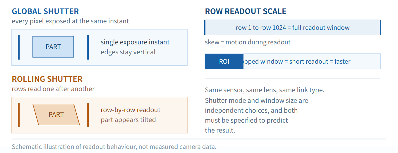
The shutter mode determines whether a fast-moving object appears where it actually was. A global shutter exposes all pixels simultaneously and then reads them out; a rolling shutter exposes and reads row by row, so a moving part appears tilted or stepped. In a high-speed SWIR InGaAs camera used for production inspection, a skewed silhouette can defeat a feature-extraction algorithm even when the blur itself is negligible. Every camera discussed here specifies a global shutter, and that is the default choice for anything that moves.
Rolling shutter is not a defect; it is a trade that suits static scenes. If a vendor offers two options for the shutter mode on one SWIR camera, ask which one produces the published frame rate, because the two figures are rarely the same.
Minimum exposure time and the frame period budget
The minimum exposure time is the shortest gate a SWIR InGaAs camera can open, and it defines how fast the scene may move before it smears. A 1.3 MP 400–1700 nm InGaAs camera with a 5 μm pixel supports a 15 µs minimum exposure and a range up to 60 s; the same floor appears on the 5 MP variant. A 1.3 MP 15 μm model runs 16 µs to 1 s on USB3.0 and CameraLink, and 25 µs to 5 s on its 10GigE version — a consequence of the readout path, and the detail that decides whether a moving part stays sharp.
Budget the frame period properly. The usable period equals the exposure plus the readout plus transfer and processing overhead, and the minimum exposure time has to fit inside it. A 200 fps camera gives a 5 ms frame period; at 15 µs the remaining 4.985 ms is readout and transfer. Push the exposure to 1 ms and the same camera drops to roughly 970 fps. Long exposure and high frame rate cannot coexist on one SWIR camera.
Windowing mode and region-of-interest readout
Windowing mode turns a SWIR InGaAs camera from a moderate full-frame rate into a headline rate. Implemented as a hardware region-of-interest readout, it digitises only the pixels inside the window, so the readout time falls roughly in proportion to the area left out. The single-zone ROI in AttosView supports a maximum of 8000 fps after cropping, while the full-frame rate on the same sensor is 200 fps at 1280 × 1024.
Treat that ratio as a spatial contract rather than a camera headline. If the measurement needs only a 512 × 512 patch on a moving part, 8000 fps is real and repeatable; if you need the whole field, you are back to full-frame throughput, and the interface has to carry it. Cropping also changes the optics: the effective focal length does not change, but the usable field of view does, so a lens selected for the full sensor no longer frames the same scene. Windowing mode buys frame rate with field of view, so ask for the rate at the window size you will actually use.
Dynamic range, gain and what a fast frame can hold
Dynamic range is the span between the darkest signal that rises above the noise floor and the level at which the pixel saturates. In a SWIR InGaAs camera it is set by full-well capacity against read noise and conversion gain, and it is the attribute that suffers most when you push speed. The 1.3 MP 5 μm InGaAs camera holds 181.6 ke of full well against 211 e of readout noise and a 44.3 e/ADU conversion gain, giving 58.7 dB and a maximum SNR of 52.6 dB. The 5 MP 3.45 μm model reaches 51.36 dB in high-conversion-gain mode, with a smaller 41.39 ke full well.
Two habits protect the dynamic range you paid for. Use the gain range deliberately — both A-series cameras offer 1× to 15× — and prefer the lowest gain that still resolves the feature, because gain amplifies noise as well as signal. And where a shiny metal sits against a dark background, a single exposure cannot hold both: capture an unsaturated low-gain frame and a high-gain frame at a different exposure time and merge them, while the hardware ROI concentrates the dynamic range on the region that matters. At high frame rates that costs time, because the two frames are sequential.
Interface bandwidth, buffering and triggering
The link decides the practical frame rate of a SWIR InGaAs camera, and it is the first thing to fix when the sensor falls short of its quoted speed. The same 1.3 MP array is offered across USB3.0, GigE, CoaXPress and CameraLink, with identical imaging performance across the four — only the transport differs. USB3.0 is plug-and-play for a lab bench; GigE or 10GigE carries the signal over long cable runs on a production line; CoaXPress is the high-bandwidth option for semiconductor defect inspection and needs a matching capture card; CameraLink fits established research platforms.
Two supporting details make the difference at speed. A 512 MB image buffer absorbs the burst between acquisition and processing, so a frame is not dropped while the host is still working, and external triggering with configurable delay lets the camera fire exactly when the encoder says so. Choose the interface before you compare sensors, because it caps the rate any SWIR camera can deliver. Confirm the shutter mode is global on the model you order, and check the digital I/O: one optically isolated input, one optically isolated output and two non-isolated channels cover most lines.
Sensor temperature and the dark current it controls
Dark current is the noise floor that rises with temperature, and at high speed it competes directly with the signal in every short frame. A TEC-cooled InGaAs camera holds the sensor roughly 25 °C below ambient — about -10 °C at a 20 °C ambient — with PID control and a 0.3 °C deviation. That brings dark current down to 383 e/s at 0 °C from 638 e/s at 20 °C on the 1.3 MP model. A 1.5″ 15 μm design pushes further, to 40 °C below ambient, at the cost of a larger body.
Read the power number alongside the cooling number. The 1.3 MP 5 μm unit draws under 25 W with refrigeration active; the 15 μm 1.3 MP model runs at 8.4 W with the TEC off and under 16 W with it on. A SWIR InGaAs camera that has to sit in a sealed enclosure or run from a battery needs that balance resolved before the camera is chosen, and no shutter mode setting changes it.
| Attribute | What it controls | What to verify on the datasheet |
|---|---|---|
| Shutter mode | Whether moving parts stay in place | Global shutter confirmed at the quoted rate, not a rolling option |
| Minimum exposure time | Motion blur and pulse capture | Shortest gate in µs, and the exposure range around it |
| Frame period | Realistic frame rate | Full-frame rate and the readout time that supports it |
| Windowing mode | Speed after cropping | ROI frame rate quoted at your window size, not the smallest supported |
| Dynamic range | Contrast a single frame can hold | Full well, read noise, conversion gain and the figure per gain mode |
| Interface and buffering | Whether frames arrive intact | Link type, capture card requirement, buffer size, trigger and I/O levels |
Best-in-class high-speed SWIR cameras with few compromises
Few compromises does not mean every specification is maximal. It means the trade-offs left on the table are ones your process will never touch. Three SWIR InGaAs cameras in the AttosTek catalogue make that trade differently, and each keeps the same four attributes intact — global shutter, a 15 µs-class minimum exposure, hardware windowing and a documented dynamic range. A SWIR camera that is fast on paper and slow in the rack is not the answer.
The 1.3 MP 5 μm model: the balanced choice
The SWIR051A series is built on the Sony IMX990 sensor at 1280 × 1024 with 5 μm pixels, covering 400–1700 nm. It holds 200 fps at full resolution and reaches 8000 fps in windowing mode, with a 15 µs minimum exposure time, a range up to 60 s, 512 MB of buffer and 58.7 dB of dynamic range — the highest of the three. A 12-bit ADC with optional 8-bit and 10-bit output, 181.6 ke of full well, 211 e of readout noise and a 44.3 e/ADU conversion gain sit underneath that. It weighs under 390 g, mounts C-mount, draws under 25 W with the TEC running, and comes in USB3.0, GigE, CoaXPress and CameraLink variants. The 1.3 MP 5 μm 400–1700 nm TEC-cooled SWIR InGaAs camera is the configuration most high-speed SWIR camera buyers end up on, because it balances pixel pitch, dynamic range and thermal budget without giving up anything that matters at 200 fps.
The 5 MP 3.45 μm model: resolution when the field is wide
The SWIR035A series uses the Sony IMX992 at 2560 × 2048 with 3.45 μm pixels over the same 400–1700 nm band. It keeps the 15 µs to 60 s exposure range, the global shutter, 512 MB of buffer, 1× to 15× gain and the same four interface options including 10GigE and CoaXPress. The cost is per-pixel headroom: 41.39 ke of full well in high-conversion-gain mode against 111.88 e of readout noise, giving 51.36 dB of dynamic range and a 46.17 dB maximum SNR. Smaller pixels gather less light, so a scene comfortable for the 5 μm sensor can sit near the floor here — the price of resolution in a SWIR camera. Where one frame must cover a large area of a moving part, a full wafer or a wide conveyor section, the 5 MP 3.45 μm SWIR InGaAs camera is the right tool, a deliberate trade of light per pixel for pixels per frame.
The 1.3 MP 15 μm model: sensitivity and field of view
The SWIR151B series moves the other way, to an InGaAs camera with 15 μm pixels on a 1.5″ sensor at 900–1700 nm, a 14-bit ADC and 200 fps at 1280 × 1024. Quantum efficiency reaches 70% at 1.55 μm, where the water absorption band sits, and the full well in low-conversion-gain mode reaches 1.9 Me⁻. Cooling runs 40 °C below ambient, and the body is larger — 68 × 68 × 89.8 mm at 485 g on an M42 mount — with a lower power draw: 8.4 W with the TEC off, under 16 W with it on. Where a measurement is faint and the field of view is wide, the large-pixel 1.3 MP 15 μm 900–1700 nm SWIR InGaAs camera wins on light collection and format size rather than on pixels per second.
| Parameter | SWIR051A — 1.3 MP, 5 μm | SWIR035A — 5 MP, 3.45 μm | SWIR151B — 1.3 MP, 15 μm |
|---|---|---|---|
| Sensor | Sony IMX990 InGaAs | Sony IMX992 InGaAs | InGaAs CMOS |
| Resolution | 1280 × 1024 | 2560 × 2048 | 1280 × 1024 |
| Pixel size | 5.0 μm × 5.0 μm | 3.45 μm × 3.45 μm | 15 μm × 15 μm |
| Spectral range | 400–1700 nm | 400–1700 nm | 900–1700 nm |
| Shutter mode | Global shutter | Global shutter | Global shutter |
| Exposure range | 15 µs – 60 s | 15 µs – 60 s | 16 µs – 1 s (USB3.0 / CL), 25 µs – 5 s (10GigE) |
| Full-frame frame rate | 200 fps | Not published on the product page | 200 fps at 1280 × 1024 |
| Windowing mode (ROI) | Up to 8000 fps | Hardware ROI and external triggering | Single-zone ROI, up to 8000 fps |
| Dynamic range | 58.7 dB | 51.36 dB (HCG) / 51.47 dB (LCG) | Not published on the product page |
| Full well / read noise | 181.6 ke / 211 e | 41.39 ke (HCG) / 111.88 e (HCG) | 1.9 Me⁻ (LG) / 118.75 ke⁻ (MG) |
| ADC / buffer | 12-bit (8/10 optional) / 512 MB | 12-bit / 8-bit, 512 MB | 14-bit, 512 MB |
| Cooling | 25 °C below ambient | 25 °C below ambient | 40 °C below ambient |
| Power / weight | <25 W / <390 g | <25 W / <390 g | 8.4 W (TEC off) / <16 W (TEC on), 485 g |
| Interfaces | USB3.0, GigE, CoaXPress, CameraLink | USB3.0, 10GigE, CoaXPress, CameraLink | USB3.0, 10GigE, CameraLink |
From spec sheet to shortlist: a procedure that takes one afternoon
Run these five steps in order, because each one removes options that cannot satisfy the next.
1. Write down the event, not the camera. “A 2 mm defect moving at 1.5 m/s” is a usable requirement; “fast camera” is not. Record the target size, the speed, the field of view, the lighting and the shutter mode you need — global for anything that moves. A 400–1700 nm sensor behind the standard filter passes visible light too, so the same part can be imaged in both bands.
2. Convert motion into an exposure limit. Divide your blur tolerance by the target speed and you have a maximum exposure. Below 100 µs, the 15 µs floor of the A-series models is comfortable, while the 25 µs minimum exposure time on a 10GigE model may already smear parts moving at line speed. Above 10 ms, this is not a high-speed application at all.
3. Decide whether you will crop. If the measurement needs one region only, windowing mode trades field of view for frame rate. If the whole frame must be captured, work with the full-frame rate and size the interface to it: a 200 fps stream at 1280 × 1024 with 12-bit data runs at roughly 3.1 Gbit/s before overhead, and that figure decides whether the SWIR camera on your shortlist can keep up with the line.
4. Set the noise floor from the scene. Decide the illumination and the shortest exposure, compute the photon count in that exposure, and compare it with the read noise of the candidate InGaAs camera: 211 e on the 1.3 MP 5 μm model, 111.88 e in high-conversion-gain mode on the 5 MP model. If the photon count sits far below the read noise, more pixels do not help — a larger pixel does. Check the shutter mode while you are there: a rolling sensor adds skew that no gain setting can remove.
5. Match the interface to the host. Then check cooling and power against the enclosure, the mounting against the fixture, and the software against your stack. AttosView covers camera control, acquisition, processing and analysis; the SDK covers native C/C++, .NET with C# and VB.NET, Python, Java, DirectShow, TWAIN, LabVIEW and MATLAB, on Win32, WinRT, Linux, macOS and Android. Integration effort, not SWIR camera price, is what makes a project late.
AttosTek builds across the whole 1–14,000 nm range, so a multi-band programme — short-wave infrared for material contrast, thermal bands for temperature — can be specified as one system, with the SWIR InGaAs camera selected as the short-wave element of it. Where a catalogue model does not fit, the AttosTek customization team configures sensor, interface, cooling and housing for small batches and returns a CIF quotation. The wider InGaAs and CQD SWIR camera range covers uncooled and deep-cooled variants when speed is not the binding constraint.
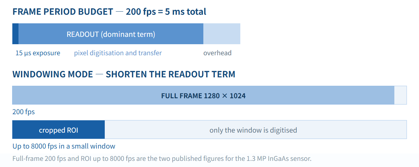
High-Speed SWIR InGaAs Cameras from AttosTek
The four models below cover the configurations discussed in this article — from the 1.3 MP SWIR camera that reads the full array at 200 fps and climbs to 8000 fps in windowing mode, to an uncooled 70 g unit for portable instruments. Every SWIR camera ships with AttosView control software, a full SDK and CE/FCC certification.
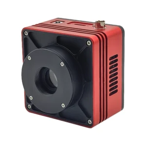 1280 × 1024 @ 200 fps full frame · ROI up to 8000 fps · 58.7 dB dynamic range · 15 µs–60 s exposure · 400–1700 nm · USB3.0 / GigE / CoaXPress / CameraLink
|
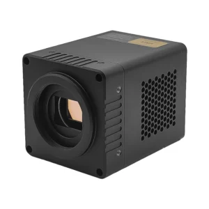
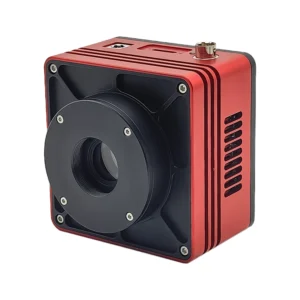 2560 × 2048 at 3.45 µm pixels · 51.36 dB dynamic range (HCG) · 15 µs–60 s exposure · global shutter · USB3.0 / 10GigE / CoaXPress / CameraLink
|
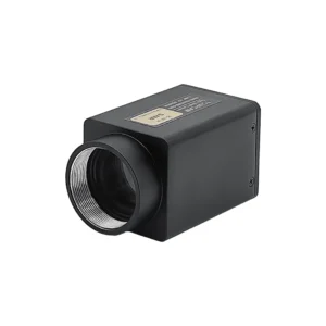
 15 µm pixels on a 1.5″ sensor · QE ≥ 70% at 1.55 µm · 200 fps at 1280 × 1024 · 40 °C below ambient · USB3.0 / 10GigE / CameraLink
|
 Bus-powered at under 2.11 W · 33 × 33 × 38 mm, 70 g · plug-and-play for portable and OEM instruments · 400–1700 nm
|
Why Buyers Choose AttosTek for High-Speed SWIR Imaging
|
Complete Product Range
Cooled, uncooled and deep-cooled SWIR cameras plus UV-VIS, MWIR and LWIR lines from one supplier.
|
Quality Excellence
100% factory testing before shipment, with CE and FCC certification on every camera.
|
Flexible Customization
Sensor, interface, cooling and housing options, accepted even for small-batch orders.
|
Timely Service
7 × 24 support across the full lifecycle, from sensor selection through integration.
|
Frequently Asked Questions
What is the difference between windowing mode and binning?
Windowing mode reads out only the pixels inside a selected rectangle, so the frame rate rises as area is removed. Binning merges neighbouring pixels into one larger output pixel, improving signal-to-noise but softening the image. Windowing mode keeps every pixel sharp and shrinks the field of view; binning keeps the field of view and loses detail.
How fast can a high-speed SWIR InGaAs camera actually run?
On a 1.3 MP 1280 × 1024 InGaAs sensor, the full-frame rate is 200 fps and windowing mode reaches up to 8000 fps in a small region of interest. The 5 MP 2560 × 2048 model is built for resolution rather than headline speed, so request its full-frame figure on the quotation. The achievable rate is always set by the slowest link in the chain.
Does a global shutter matter for short-wave infrared inspection?
Yes, whenever the part moves. A global shutter exposes every pixel at the same instant, so a moving component keeps its true shape and position. A rolling shutter reads row by row and shows a moving part as tilted or stepped, which can defeat feature-extraction software even when the blur is small. Treat a global shutter as a requirement when comparing suppliers.
How much dynamic range do I need for my measurement?
Start from the contrast in the scene and check it against the sensor figures. The 1.3 MP 5 μm model offers 58.7 dB, the 5 MP 3.45 μm model 51.36 dB. Where a shiny metal sits next to a dark background, capture an unsaturated low-gain frame and a high-gain frame, merge them into an HDR image, and use the hardware ROI to concentrate the dynamic range on the region that matters.
Can AttosTek quote a custom interface and cooling configuration?
Yes. AttosTek supports small-batch customization covering sensor, interface, cooling, housing and lens, and every camera ships with AttosView, a multi-platform SDK and CE/FCC certification. Quotations are CIF, which includes freight and insurance but excludes destination duty, import tax and VAT; logistics is a flat 50 USD within Asia and 100 USD elsewhere.
Technical support: support@attostek.com · (+86) 156 5912 7889


